Window Functions
import numpy as np
import matplotlib.pyplot as plt
import librosa
import IPython.display as ipd
Non-Integer Frequencies
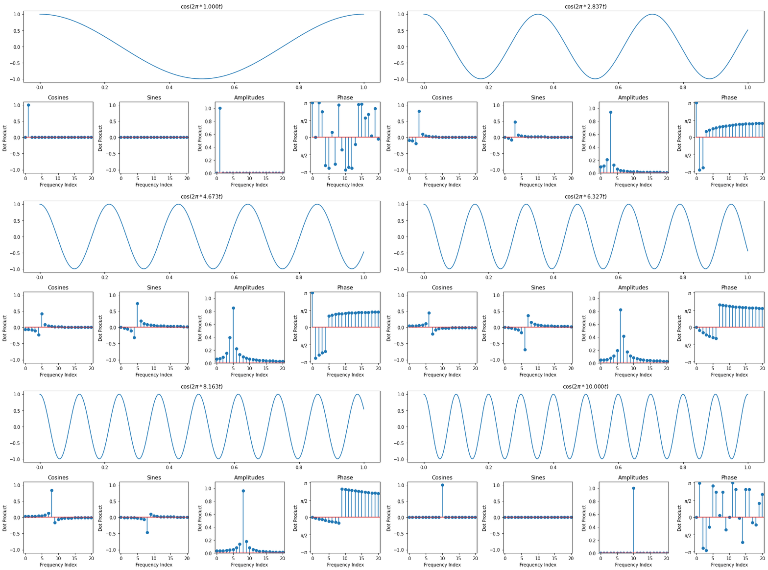
Recall how we ran into an interesting situation even with a pure cosine when the frequency wasn't a whole number
The Periodicity Assumption
When we derived the discrete fourier transform, one of our key assumptions behind each frequency was that it went through a whole number of periods over the interval we were looking at. This was crucial to ensure that the dot products were 0 for different frequencies. Another way to understand this assumption is to envision our signal as living on a circle. Since it has to immediatly pick up again where it left off, it can be thought of as looping around
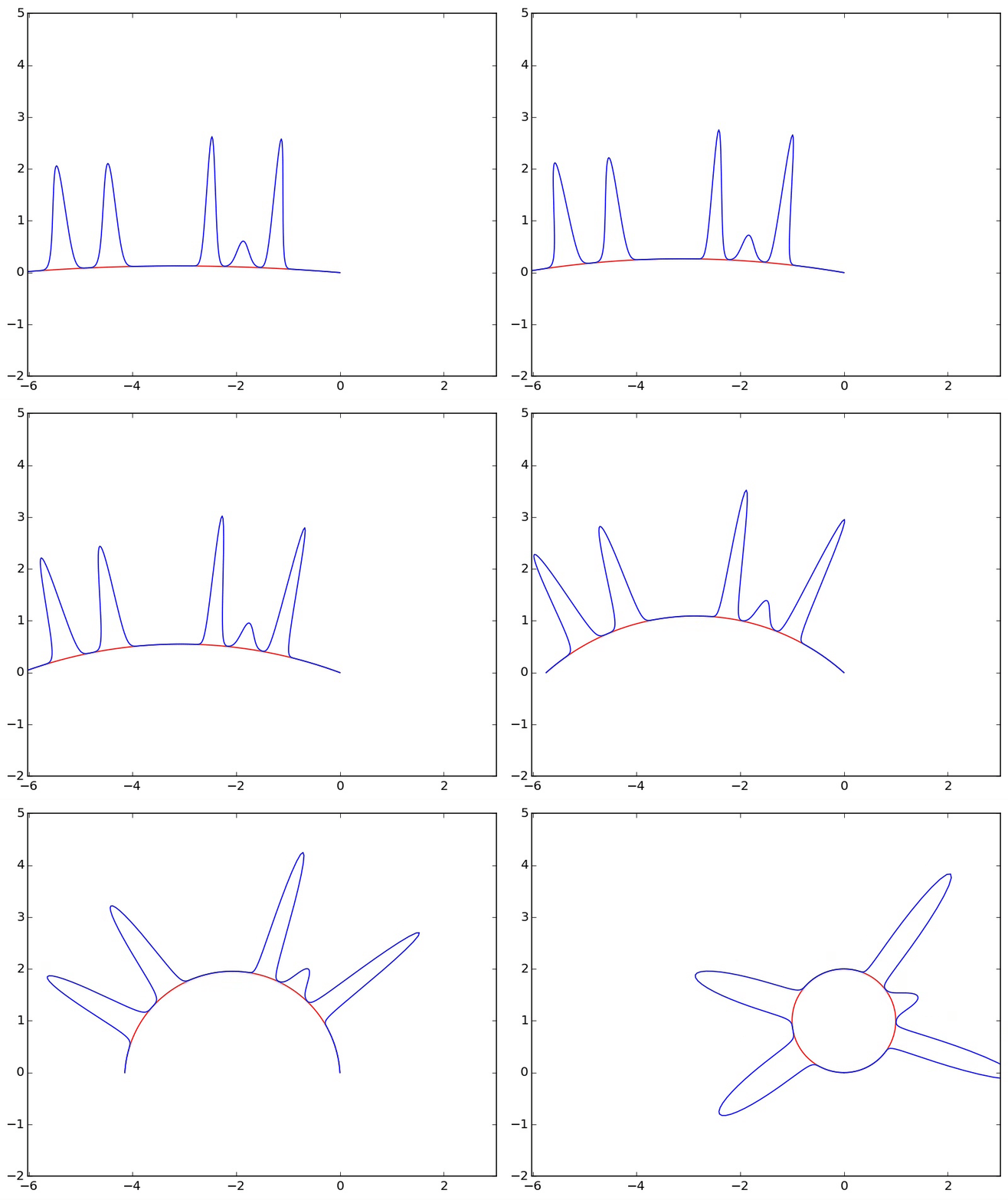
In this context, a phase shift is simply a rotation, which is already mind blowing
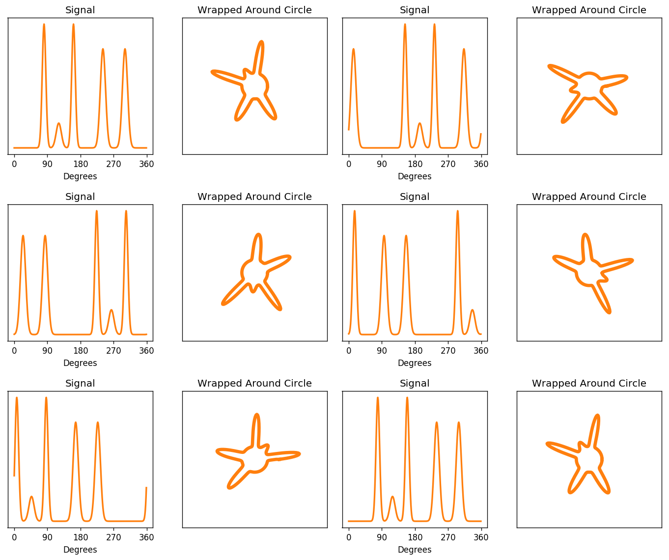
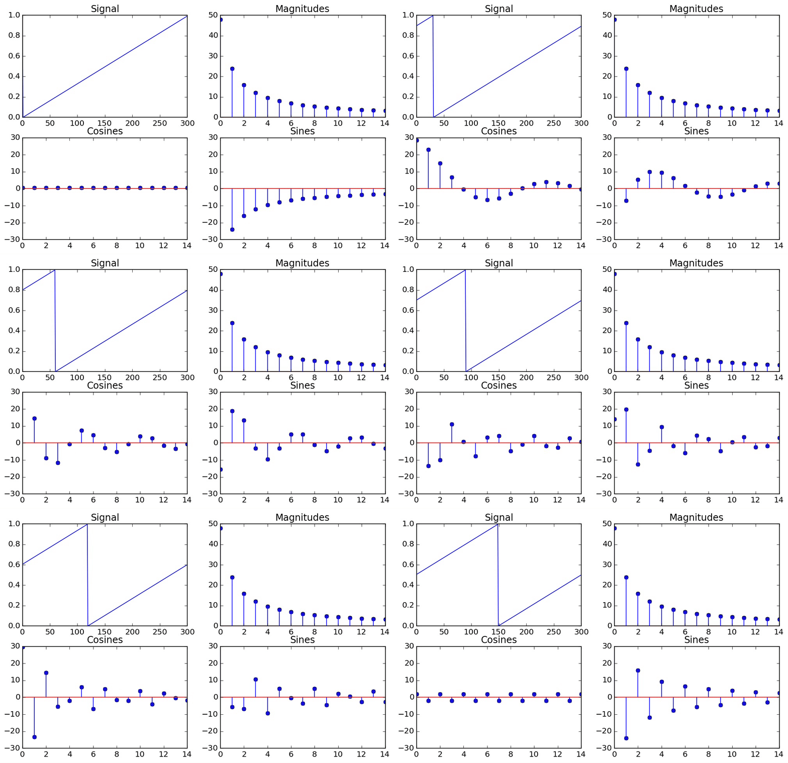
Another way to look at this is that we're taking a window of a longer signal that is infinitely periodic, with a whole number of periods occuring in the length of the window
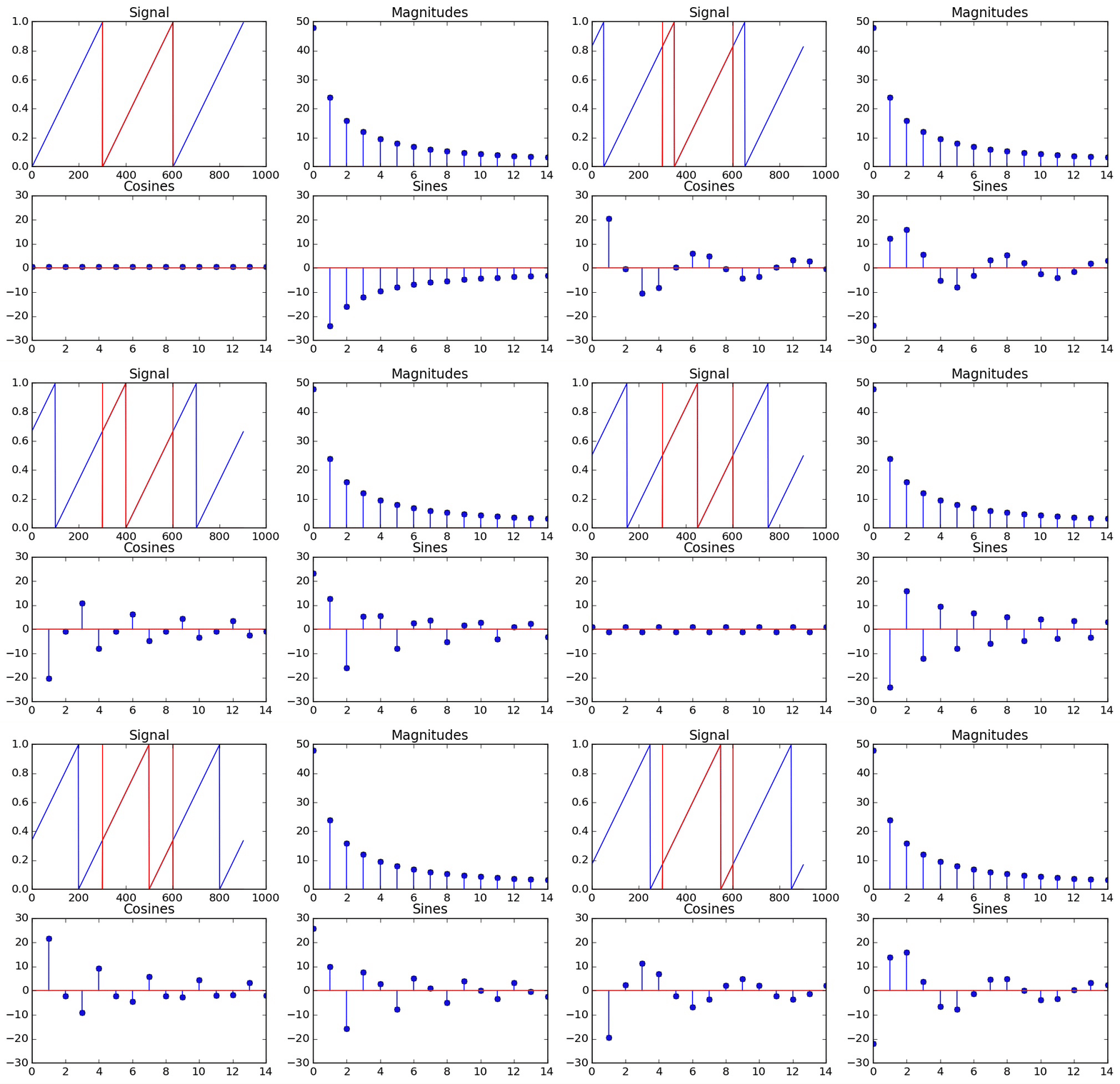
The Effect of Windowing
If we take a window of a signal which goes through a whole number of periods in that window, then we get results that we expect
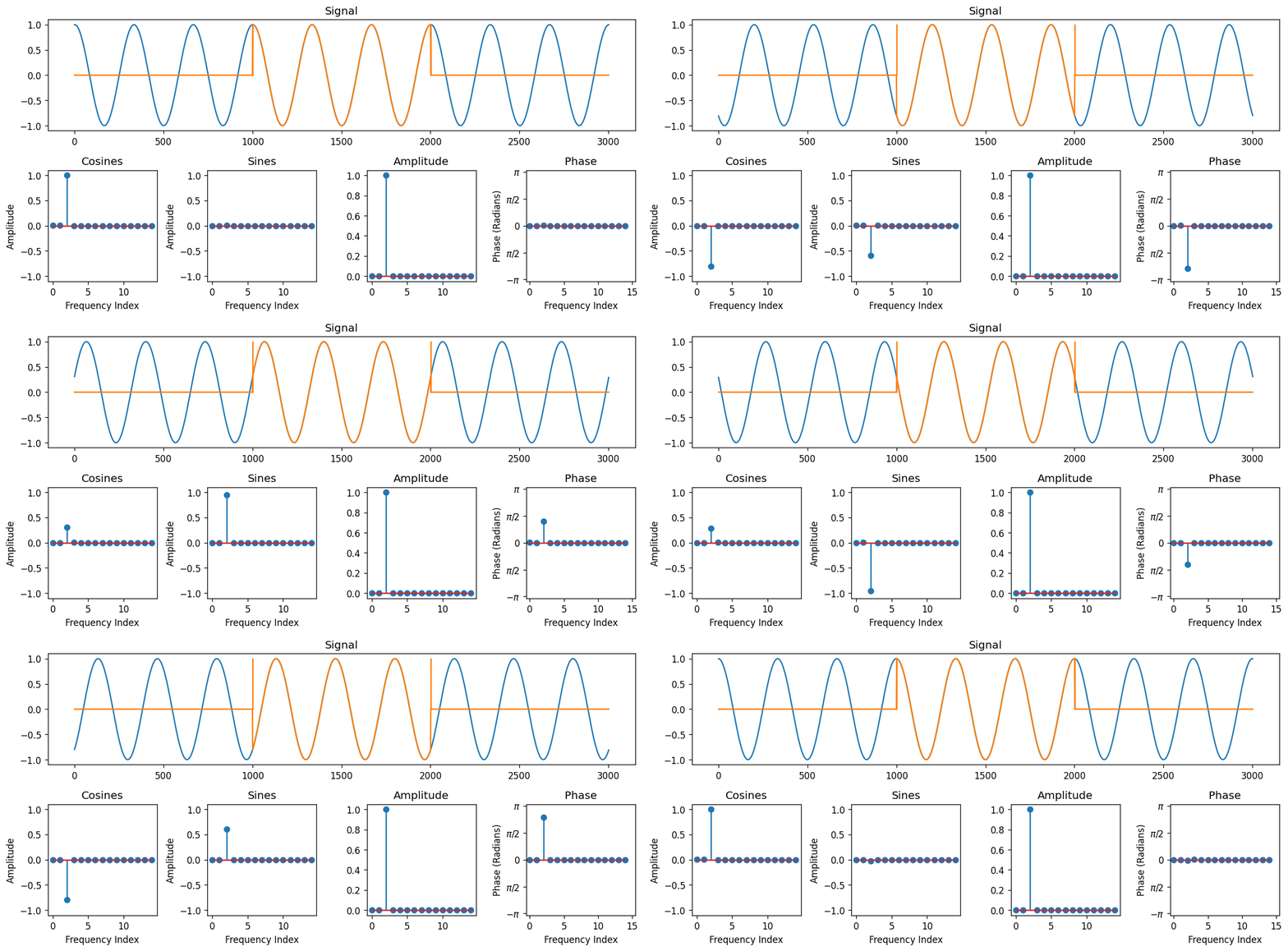
However, if we take a signal which does not go through a whole number of periods, then the DFT is actually assuming that it does repeat itself perfectly periodically at the end, so we end up seeing that it's a window of an infinitely periodic function that jumps abruptly from one period to the next. In general, when there are jumps in a signal, we need high frequencies to represent it. So this explains why we need so many frequencies to represent what seemed at a first glance like a pure cosine
N = 100
window_fn = np.sin(np.pi*np.arange(N)/N)
plt.plot(window_fn)
In other words, we take
$x_w[i] = x[i]*\sin(\pi i / N)$
If we return to our example of the cosine going through a non-integer number of periods, we see the following effect
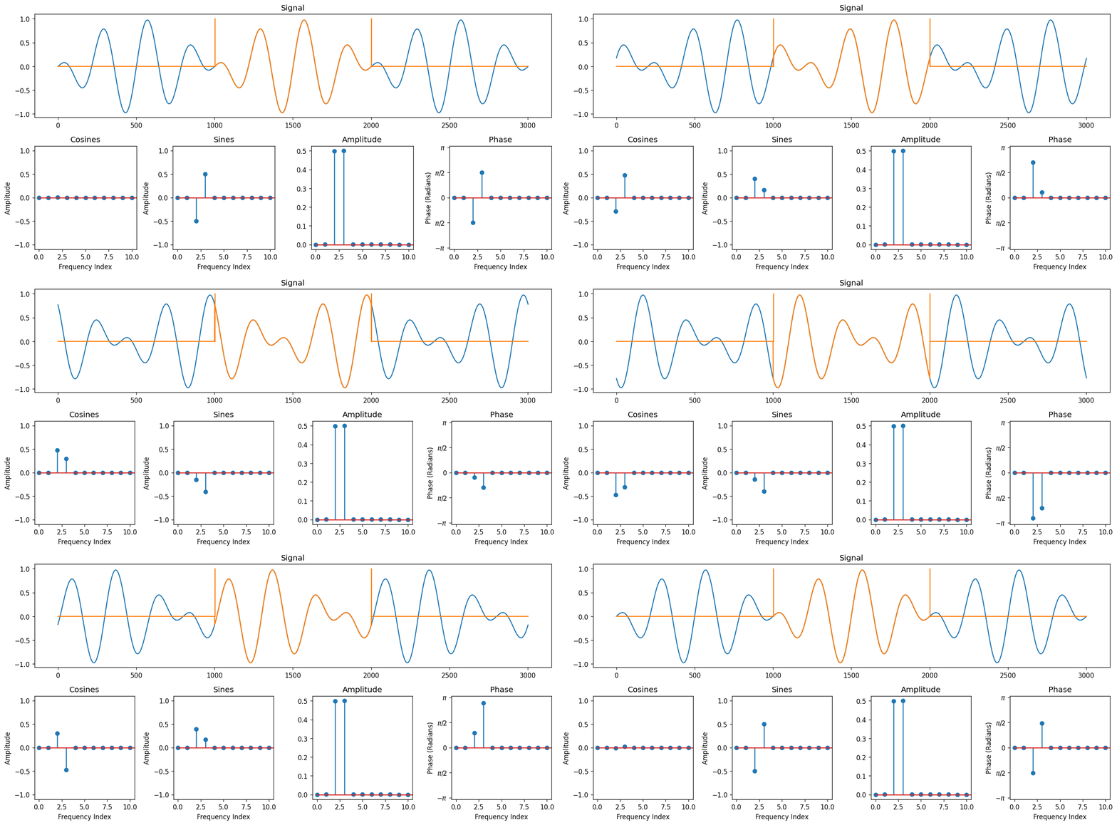
Now we only get two frequencies activated, and our signal has a frequency right in between those two.
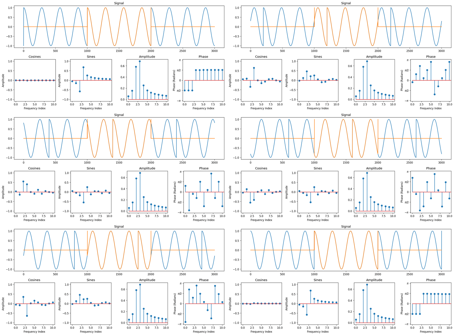
We see a similar thing with a square wave that goes through 4.5 periods over the interval. If, by the DFT assumption, it is to come as one cycle in an infinitely periodic sequence, the effect is that one of the squares gets dragged out, and the harmonic frequencies bleed into adjacent bins in the DFT
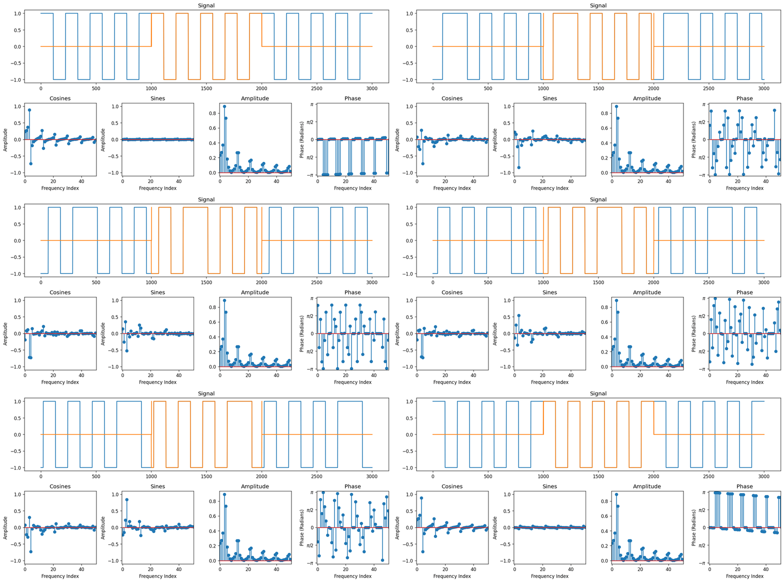
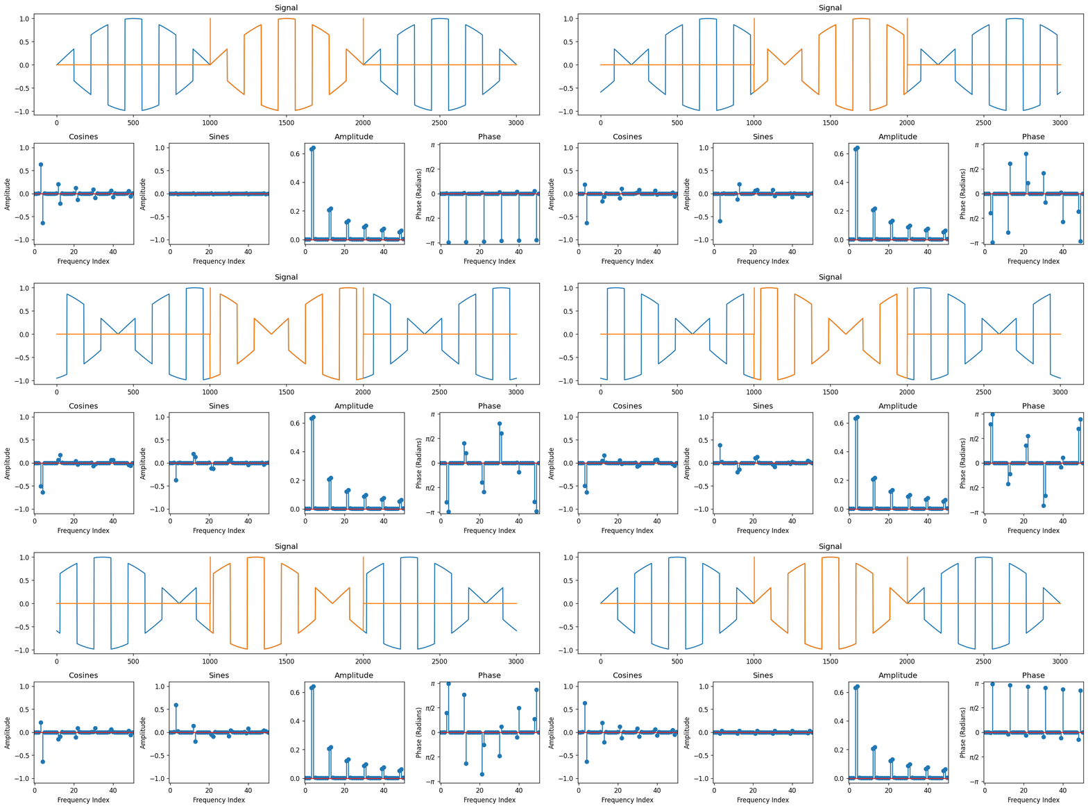
By contrast, if we apply a sine window first, we only get a significant response for the two whole number frequencies that are the closest to each harmonic
Hann Window on STFT
The window effect is more pronounced where the window is smaller and there are fewer cycles relative to where one gets chopped off, so this is a very common step in the short-time fourier transform. We're now going to look at using the Hann Window, as shown below
$f(n) = \sin^2(\pi n / N) = 0.5(1 - \cos(2 \pi n/N))$
N = 100
f = 0.5*(1 - np.cos(2*np.pi*np.arange(N)/N))
plt.plot(f)
def get_dft(x):
    """
    Return the non-redundant real/imaginary components
    of the DFT, expressed as amplitudes of sines/cosines
    involved

    Parameters
    ----------
    x: ndarray(N)
        A signal

    Returns
    -------
    cos_sum: ndarray(ceil(N/2)), sin_sums(ndarray(ceil(N/2)))
        DFT cosine/sine amplitudes
    """
    N = len(x)
    t = np.linspace(0, 1, N+1)[0:N]
    n_freqs = int(np.ceil(N/2))
    f = np.fft.fft(x)
    cos_sums = np.real(f)[0:n_freqs]/(N/2)
    sin_sums = -np.imag(f)[0:n_freqs]/(N/2)
    return cos_sums, sin_sums
def specgram(x, w, h, sr, win_fn):
    """
    Compute the "spectrogram"
    (amplitudes of the short-time fourier transfrom)
    Parameters
    ----------
    x: ndarray(N)
        Full audio clip of N samples
    w: int
        Window length
    h: int
        Hop length
    sr: int
        Sample rate

    Returns
    -------
    ndarray(w, nwindows) Spectrogram
    """
    N = len(x)
    i = 0
    nwin = int(np.floor((N-w)/h))+1
    n_freqs = int(np.ceil(w/2))
    # Make a 2D array
    # The rows correspond to frequency bins
    # The columns correspond to windows moved forward in time
    S = np.zeros((n_freqs, nwin))
    # Loop through all of the windows, and put the fourier
    # transform amplitudes of each window in its own column
    for j in range(nwin):
        # Pull out the audio in the jth window
        # Ex) First window x[0:w]
        # Ex) Second window x[h:h+w]
        # Ex) Third window x[2h:2h+w]
        xj = win_fn(w)*x[h*j:h*j+w]
        # Do the fourier transform of the jth window
        c, s = get_dft(xj)
        amps = np.sqrt(c**2 + s**2)
        # Put the fourier transform amplitudes into S
        S[:, j] = amps
    return S
def hann_window(N):
    return 0.5*(1 - np.cos(2*np.pi*np.arange(N)/N))
x, sr = librosa.load("chromatic2octaves.wav", sr=44100)
win = 2048*2
hop = 256
win_fn = lambda N: 1
#win_fn = hann_window
S = specgram(x, win, hop, sr, win_fn)
times = hop*np.arange(S.shape[1])/sr
freqs = np.arange(S.shape[0])*sr/win
S = np.log10(S/np.min(S))
plt.figure(figsize=(12, 6))
plt.imshow(S, cmap='magma_r', extent = (times[0], times[-1], freqs[-1], freqs[0]), aspect='auto', interpolation='none')
plt.ylim([3000, 0])
plt.gca().invert_yaxis()
plt.colorbar()
x, sr = librosa.load("chromatic2octaves.wav", sr=44100)
win = 2048*2
hop = 256
win_fn = hann_window
S = specgram(x, win, hop, sr, win_fn)
times = hop*np.arange(S.shape[1])/sr
freqs = np.arange(S.shape[0])*sr/win
S = np.log10(S/np.min(S))
plt.figure(figsize=(12, 6))
plt.imshow(S, cmap='magma_r', extent = (times[0], times[-1], freqs[-1], freqs[0]), aspect='auto', interpolation='none')
plt.ylim([3000, 0])
plt.gca().invert_yaxis()
plt.colorbar()
As you can see, the Hann window makes the harmonics jump out more against the background, and there isn't as much bleed between the harmonics