Aliasing
import numpy as np
import matplotlib.pyplot as plt
import IPython.display as ipd
import librosa
Recall that frequencies are mirror images of each other after roughly $N/2$
N = 40
plt.figure(figsize=(20, 15))
for k in range(N):
    c = np.cos(2*np.pi*k*np.arange(N)/N)
    s = np.sin(2*np.pi*k*np.arange(N)/N)
    plt.subplot(N, 2, k*2+1)
    plt.plot(c)
    plt.axis('off')
    plt.subplot(N, 2, k*2+2)
    plt.plot(s)
    plt.axis('off')
Real part is the same for frequency $k$ and frequency $N-k$, but the imaginary part is the exact negation between frequency $k$ and freuqency $N-k$. What this means is that the coefficients of the complex DFT $X[k]$ and $X[N-k]$ are "complex conjugates" of each other. (Imaginary component gets flipped).
Aliasing
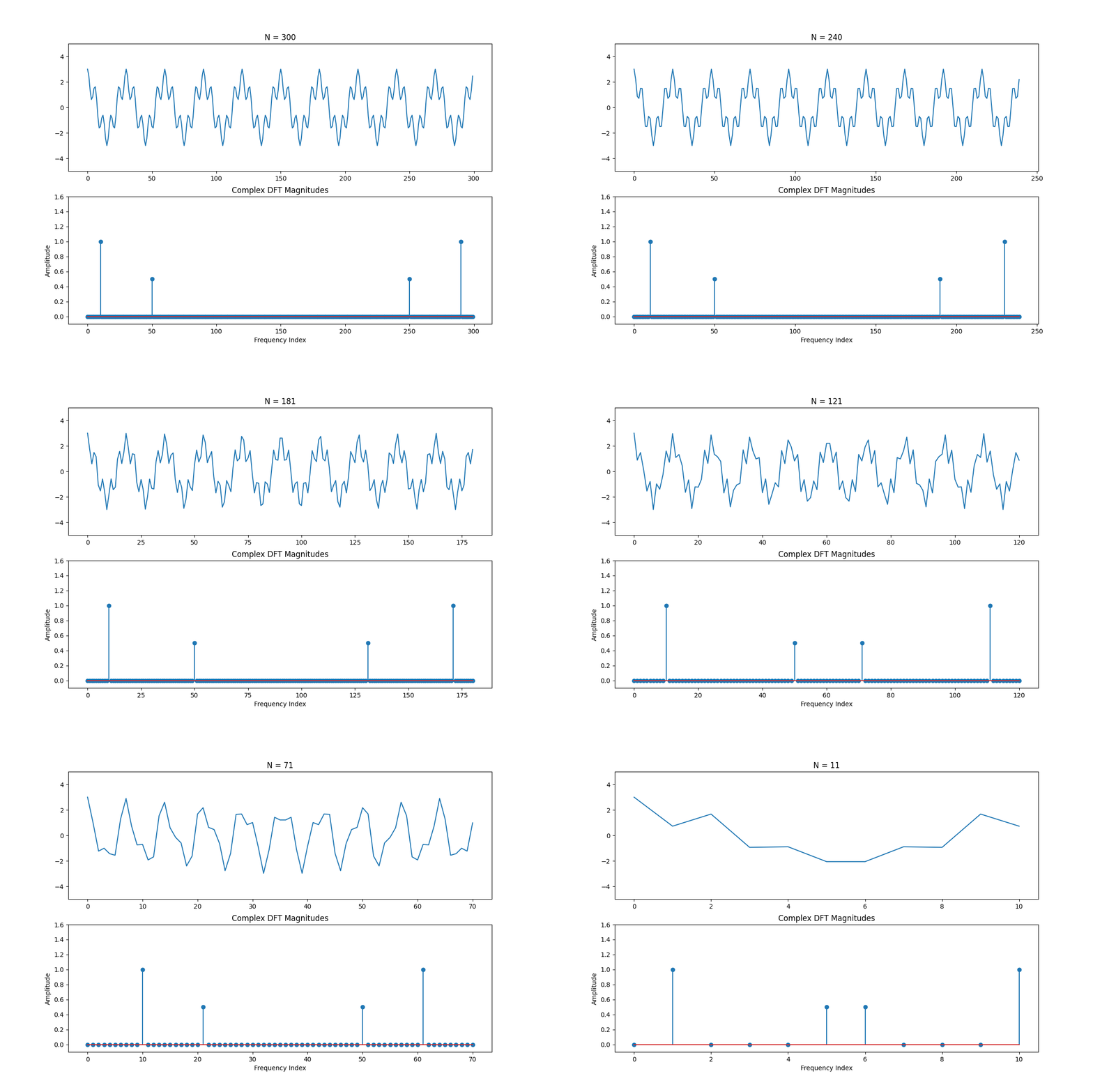
Furthermore, if we're trying to represent frequencies that are beyond half the sample rate, then they get "aliased" (mistaken for) lower frequencies

Let's look at an example of what happens when we generate a square wave and don't take enough samples. Originally, we're OK and we see all of the harmonics
sr = 44100
t = np.arange(sr*2)/sr
f = 880
x = np.sign(np.sin(2*np.pi*f*t))
plt.plot(np.arange(len(x))*(sr)/len(x), np.abs(np.fft.fft(x)))
ipd.Audio(x, rate=int(sr))
But if we drop the sample rate by a factor of 6, then some of the higher harmonics get aliased. We even hear some of them in the bass region below the fundamental frequency
fac = 6
y = x[0::fac]
plt.plot(np.arange(len(y))*(sr/fac)/len(y), np.abs(np.fft.fft(y)))
ipd.Audio(y, rate=int(sr/fac))
The same sort of thing can happen with audio, which leads towards a very strange effect when we pass through the Nyquist rate (half of the sample rate). Any frequency that is beyond the Nyquist rate is going to to alias if we don't properly filter it out before we sample
x, sr = librosa.load("real.mp3", 22050)
ipd.Audio(x, rate=sr)
y = x[0::fac]
ipd.Audio(y, rate=int(sr/fac))