Echoes (Reverb) And Convolution
Chris Tralie
In this module, we examine how to represent echoes in digital audio using something called "convolution"
import numpy as np
import matplotlib.pyplot as plt
import IPython.display as ipd
import librosa
from scipy.signal import fftconvolve
x, sr = librosa.load("ohmygodlook.mp3", sr=44100)
ipd.Audio(x, rate=sr)
In the real world, sound bounces off of objects in our environment and comes back to our ears at different times. To think of an example, let's say we had a big wall that was 50 meters in front of us. Noting that sound travels at 343 meters / sec and that it has to travel to the wall and back, it will come back to our ears at a 100meters / (343 meters/sec) delay. We can simulate this by adding the audio at a later slice in a numpy array, and we get the following result:
delay_time = 100/343
T = int(delay_time*sr)
print(T)
y = np.zeros(len(x)+T)
y[0:len(x)] = x
y[T::] += 0.5*x
ipd.Audio(y, rate=sr)
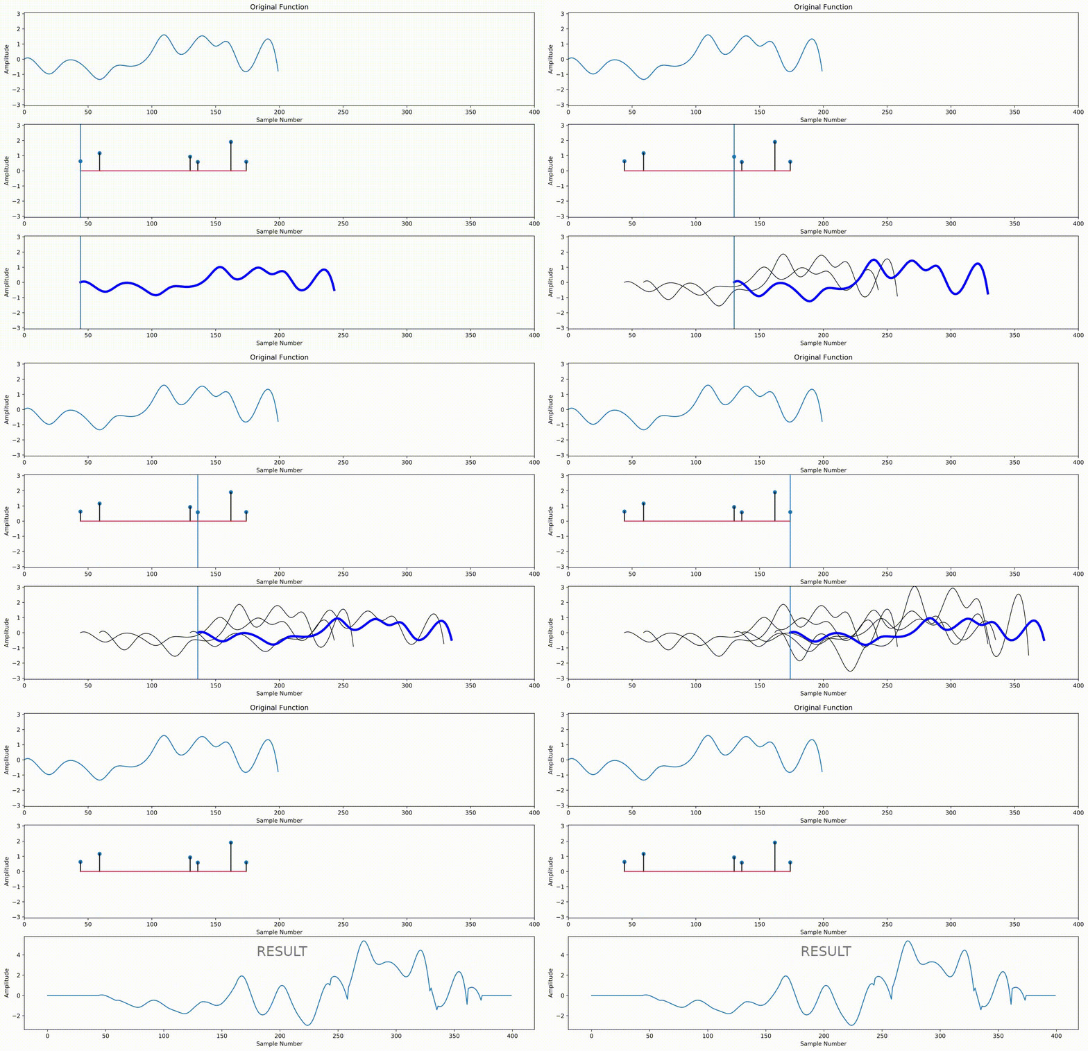
We could continue on in this fashion, but it's more convenient to define something called an "impulse response" that contains all of the echoes in our sound. Each impulse represents a different echo. Its index in the array represents the lag, and its value represents the amplitude of the echo at that lag. We simply take the entire audio we want to echo and scale it by this amplitude, shift it over by the lag, and add it to all of the other echoes to get our final result:

Below is an example of creating an impulse response, referred to as $h$, to do the same thing we did with slices a moment ago
h = np.zeros(T+1)
h[0] = 1
h[T] = 0.5
plt.plot(h)
y = np.convolve(x, h)
ipd.Audio(y, rate=sr)
Notice how we get the same result. But now it is easier with much less code to create many more echos. For instance, here is an impulse response with 5 echoes which are exponentially decaying in amplitude, which gives a neat "reverb" effect at the end
h = np.zeros(5*T+1)
h[0] = 1
h[T::T] = 0.5
h = h*np.exp(-np.arange(len(h))/(sr/2))
plt.plot(h)
y = fftconvolve(x, h)
ipd.Audio(y, rate=sr)